In This Topic
Conditional format can be set for each type of aggregation. You can specify whether to apply the format to the aggregated value including subtotal / grand totals by selecting the radio button.
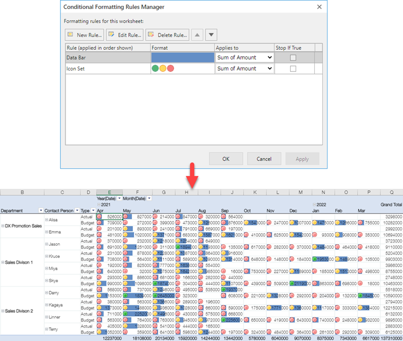
Set Conditional Format
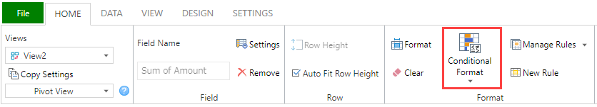
You can set the conditional format by clicking Conditional Format in the Home tab of the ribbon area. You can also set custom conditions from More Rules in the lower section of the menu or New Rule to the right of Conditional Format. For details of (1) to (5), see the respective descriptions below.
※Each conditional format has an effect depending on the field type. For details, refer to Format Field Types.
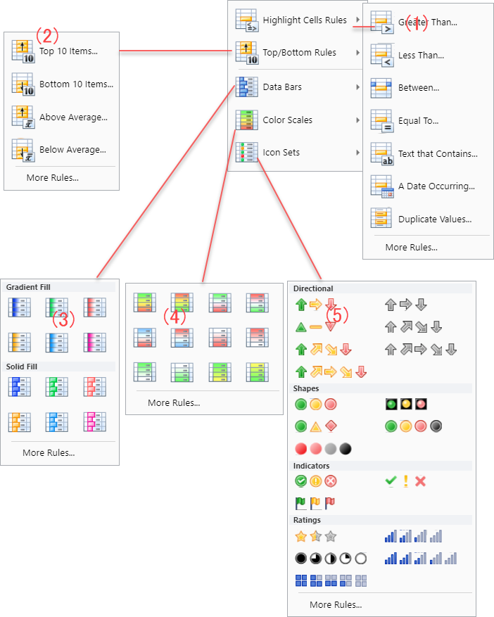
1. Highlight Cells Rules
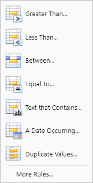
The data that satisfies one of the following rules can be highlighted.
- Greater Than...
- Less Than...
- Between...
- Equal to...
- Text that Contains...
- A Date Occuring...
- Duplicate Values...
Select one of them, and input a value or formula used to evaluate each cell. If a cell value satisfies the specified condition, the format is applied to it.
You can use the predefined highlighting style or create custom highlighting style.
2. Top/Bottom Rules
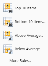
The data that satisfies one of the following rules can be highlighted.
- Top 10 Items...
- Bottom 10 Items...
- Above Average...
- Below Average...
The format is applied to the cells that have values satisfying the specified top or bottom items. As for average, the format is applied to the values that are larger or smaller than the average value in the currently displayed page.
You can use the predefined highlighting style or create custom highlighting style.
3. Data Bars
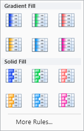
A bar is displayed in the background of each cell. The length of the bar represents its relative ratio to the values of other cells in the page. A longer data bar represents a greater value in the cell.
You can specify the value type and the value to be used as the reference.
| Percentage |
Sum of the minimum value in the cell range to which the conditional format rule is applied and the X percent of the difference between the maximum and minimum values in the cell range. For example, if the minimum and maximum values in the cell range are 1 and 10 respectively and X is 10, the value is 1.9. |
| Maximum |
The maximum value in the cell range to which the conditional format rule is applied. |
| Minimum |
The minimum value in the cell range to which the conditional format rule is applied. |
| Formula |
The result of a formula determines the minimum or maximum value of the cell range to which the rule is applied. If the operation result is not a number, it is treated as zero. |
| Percentile |
The result of the percentile function applied to the range.
|
| Automatic |
The smaller or larger, or the minimum or maximum value in the cell range to which the conditional format rule is applied.
|
| Value |
A numeric, date, or time value in the cell range to which the conditional format rule is applied.
|
Valid percentiles are from 0 to 100. You cannot use the percentile if the cell range contains more than 8,191 data points. The percentile is used to visualize a group of large values (such as the top 20 items) in one data bar and a group of small values (such as the bottom 20 items) in another data bar. It is useful when there are extremely large or small values that might skew the visualization of data.
Valid percentage values are from 0 to 100. Do not append a percent sign to the percentage value. The percentage is used to display all values linearly when the distribution of values is linear.
A formula should be prefixed with an equal sign (=). If the formula is invalid, no format is applied.
4. Color Scales
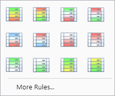
Color scales are visual guides that help you understand the data distribution and variation. A two-color scale is used to compare the values of a cell range by using a gradation of two colors. The shade of color represents higher or lower values. For example, in a green and red color scale, cells with higher values have a more green color, and cells with lower values have a more red color. You can specify the value type, value, and colors for the minimum and maximum values.
A three-color scale is used to compare the values of a cell range by using a gradation of three colors. The shade of color represents higher, middle, or lower values. For example, in a green, yellow, and red color scale, cells with higher values have a more green color, cells with middle values have a yellow color, and cells with lower values have a more red color. You can specify the value type, value, and colors for the minimum, middle, and maximum values.
5. Icon Sets
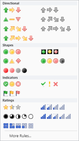
Specific icons can be displayed to indicate values larger than, equal to, or less than the specified value.