Conditional Formatting of Pivot Table
In This Topic
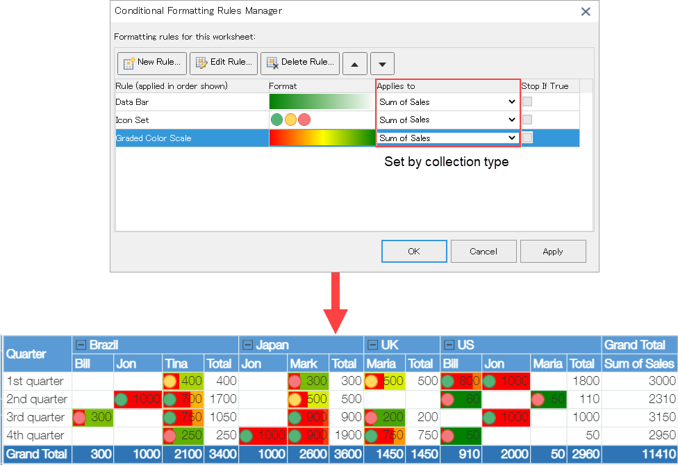
Conditional formatting is set for each type of aggregation, and formatting is applied to calculated values excluding subtotals and totals.
Apply Conditional Formatting
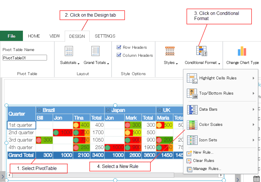
You can apply conditional formatting by clicking the Conditional Formatting option in Design tab of ribbon area. Rules are discussed in detail below.
Highlight Cells Rules
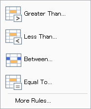
You can highlight the data that matches any of the following conditions.
- Greater than a specified value
- Lesser than a specified value
- Within a specified range
- Equal to a specified value
Select one of the above and enter a value or formula to compare each cell. If cell value meets the specified condition, the format is applied.
You can use the predefined highlighting styles or you can create your own highlighting styles.
Top/Bottom Rules
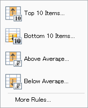
You can highlight the data that matches any of the following conditions.
- Specified top n items
- Specified bottom n items
- Above average
- Below average
Format is applied to cells having values that correspond to the specified percentage of top or bottom. Average is applied to values above or below the average value within the displayed page.
You can use the predefined highlighting styles or you can create your own highlighting styles.
Data Bars
Shows a bar in the background of each cell. Length of the bar indicates its relative ratio to the values of other cells on that page. The longer the data bar, the larger the value in the cell.
You can specify the type of base value and the value for comparison.
| Percentage |
The minimum value in the cell range to which the conditional formatting rule applies, plus X percent of the difference between the maximum and minimum values in this cell range. For example, if the minimum value in the cell range is 1, the maximum value is 10, and X is 10, the value is 1.9. |
| Maximum value |
Maximum value in the cell range to which conditional formatting rule applies. |
| Minimum value |
Minimum value in the cell range to which conditional formatting rule applies. |
| Percentile |
Result of percentile function applied to the range. |
| Automatic |
Smaller or larger value, or minimum or maximum value in the cell range to which the conditional formatting rule applies. |
| Number value |
Number, date, or time value in the cell range to which the conditional formatting rule applies. |
Valid percentiles are 0 (zero) to 100. Percentiles cannot be used if number of data points in the cell range exceeds 8,191. Percentiles are used when one data bar displays a group of large values (such as the top 20) and the other data bar displays a group of small values (such as the bottom 20). This feature is useful when the data display is distorted due to extremely large or small values.
Valid percentage values are 0 (zero) to 100. Percent sign is not used for percentage values. Percentage values are used to display all values proportionally when the distribution of values is proportional.
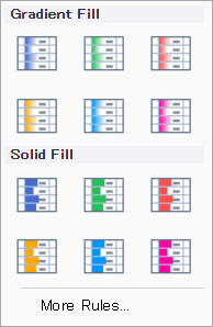
Color Scales
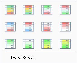
Color scale is a visual guide to understand the distribution and variation of values. The two-color scale uses a two-color gradient to compare values in a range of cells where depth of color indicates high and low values. For example, for green and red color scales, cells with higher values are drawn closer to green and cells with lower values are drawn closer to red. You can specify the value type, value, minimum value color, and maximum value color.
The 3-color scale uses a 3-color gradient to compare values in a range of cells. Color depth indicates the high, medium, and low values. For example, for green, yellow, and red color scales, higher values draw cells closer to green, intermediate values draw yellow, and lower values draw cells closer to red. You can specify the value type, value, minimum value color, intermediate value color, and maximum value color.
Icon Sets
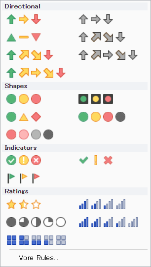
You can display a specific icon for a value greater than, equal to, or less than a specified value.
New Rule
You can specify your own condition using New Rule... option. Following example shows how to set a rule using formula and changes color of row having "Xerox Paper" as value of Dropdown_3 field.
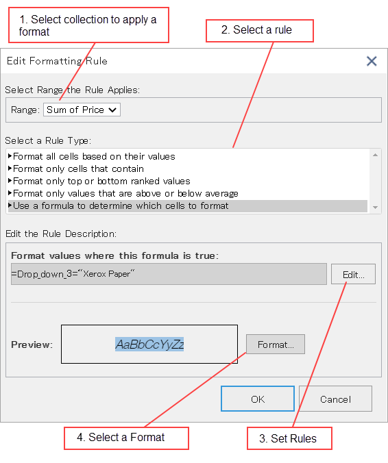
- Only kintone field set in the row can be used in the formula.
- Only field values can be referenced in formulas, not calculated values.
See Also